NLP-Based Grant Analysis

Exploratory Analysis of NSF Standard Grants Using NLP and Data Visualization Tools

---

[Back to index]

This is a small example of visualisation of the occurrence of selected keywords in the scientific abstracts of grant proposals in different research fields / directorates. It relies only on pandas, numpy, matplotlib and seaborn.

import pandas as pd
import numpy as np
import matplotlib.pyplot as plt
import seaborn as sns

Load the data to a Pandas dataframe and check the structure and headings of the data.

df = pd.read_csv('./nsf-standard-grants.csv.xz', index_col=0, encoding='utf-8')
df.head()

	year	instrument	directorate	division	abstract	funding
0	2008	Standard Grant	Directorate For Engineering	Div Of Civil, Mechanical, & Manufact Inn	NSF Proposal # 0800628: Management in Supply C...	281167.0
1	2008	Standard Grant	Direct For Computer & Info Scie & Enginr	Division Of Computer and Network Systems	Proposal Summary: The Association for Computin...	20200.0
2	2008	Standard Grant	Directorate For Engineering	Div Of Civil, Mechanical, & Manufact Inn	The research objective of this Grant Opportuni...	177948.0
3	2008	Standard Grant	Directorate For Engineering	Div Of Civil, Mechanical, & Manufact Inn	Abstract <br/>The research objective of this a...	222600.0
4	2008	Standard Grant	Directorate For Engineering	Div Of Civil, Mechanical, & Manufact Inn	This research will lead to advanced, functiona...	309973.0

We clean up the list of directorates as in the previous notebook.

dir_map = {
    'Dir for Tech, Innovation, & Partnerships': 'Tech, Innovation, & Partnerships', 
    'Direct For Biological Sciences': 'Biological Sciences', 
    'Direct For Computer & Info Scie & Enginr': 'Computer & Information Science & Engineering', 
    'Direct For Education and Human Resources': 'Education', 
    'Direct For Mathematical & Physical Scien': 'Mathematical & Physical Sciences', 
    'Direct For Social, Behav & Economic Scie': 'Social, Behavioral & Economic Sciences', 
    'Directorate For Engineering': 'Engineering', 
    'Directorate For Geosciences': 'Geosciences', 
    'Directorate for Computer & Information Science & Engineering': 'Computer & Information Science & Engineering', 
    'Directorate for STEM Education': 'Education', 
    'Directorate for Social, Behavioral & Economic Sciences': 'Social, Behavioral & Economic Sciences', 
    'Office Of Polar Programs': 'Geosciences', 
    'Office Of The Director': 'Office Of The Director'
}

df['directorate'] = df['directorate'].map(dir_map)
df.dropna(subset=['abstract'], inplace=True)
df.groupby('directorate').count()['abstract']

directorate
Biological Sciences                             10594
Computer & Information Science & Engineering    18407
Education                                       10024
Engineering                                     26773
Geosciences                                     13160
Mathematical & Physical Sciences                20218
Office Of The Director                           1708
Social, Behavioral & Economic Sciences          12071
Tech, Innovation, & Partnerships                 3495
Name: abstract, dtype: int64

We filter out directorates that contain less than 5000 abstracts.

df = df.groupby('directorate').filter(lambda x : len(x) >= 5000)

Let’s focus the examination on abstracts between years 2008 and 2022.

sel_years = list(range(2008, 2023))

We perform a heatmap visualisation of the proportion of abstracts that contain a given keyword in different years and directorates. We define two helper functions, pivot_years and heatmap_years, which create and display the heatmap, respectively. Square root is applied to all the values in the pivot table to help visualise differences between small and large values in the heatmap.

def pivot_years(kw):
    df['kw'] = df.abstract.str.contains(kw, case=False).map({True:1, False:0})
    pivot = df[df.year.isin(sel_years)].pivot_table(index='directorate', columns='year', values='kw', fill_value=0, aggfunc='mean', margins=True)
    pivot.drop('All', axis=0, inplace=True)
    pivot.sort_values('All', ascending=False, inplace=True)
    pivot.drop('All', axis=1, inplace=True)
    return pivot.apply(np.sqrt)

def heatmap_years(kw, cmap, ax):
    sns.heatmap(data=pivot_years(kw), cmap=cmap, ax=ax, square=True, cbar=False, yticklabels=True, annot=False)
    ax.set_title(kw)

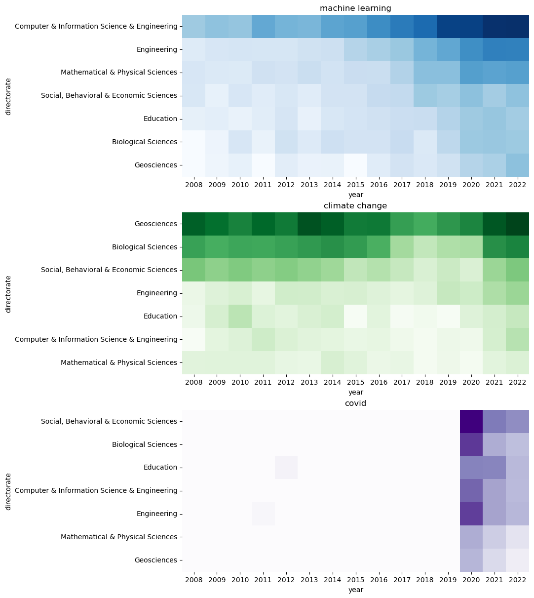
Below is a visualisation of a few select keywords. It is probably not so surprising that machine learning has been most prominent in the abstracts of Computer & Information Science & Engineering directorate and it seems to be still on the rise. Similarly, climate change has occurred most frequently in Geosciences and Biological Sciences. As a third example, covid has really appeared in abstracts only after 2020 (there are some false hits before year 2020: some projects have been sponsored by a health care products company called Covidien before the outbreak of the pandemic).

fig, (ax1, ax2, ax3) = plt.subplots(3, figsize=[12,12], constrained_layout=True)
heatmap_years('machine learning', 'Blues', ax1)
heatmap_years('climate change', 'Greens', ax2)
heatmap_years('covid', 'Purples', ax3)
plt.plot();

[Back to index]